Which Of The Harrah's Data Applications Are Most Likely Implemented Using Neural Networks?

Perceptron: Explanation, Implementation and a Visual Example

Understanding the edifice block of Neural Networks

The perceptron is the building block of bogus neural networks, it is a simplified model of the biological neurons in our brain. A perceptron is the simplest neural network, one that is comprised of merely ane neuron. The perceptron algorithm was invented in 1958 by Frank Rosenblatt.

Below is an illustration of a biological neuron:

Image by User:Dhp1080 / CC Past-SA at Wikimedia Commons

The majority of the input bespeak to a neuron is received via the dendrites. There are virtually ane,000 to ten,000 connections that are formed by other neurons to these dendrites. The betoken from the connections, chosen synapses, propagate through the dendrite into the prison cell trunk. The potential increases in the cell body and once it reaches a threshold, the neuron sends a spike along the axon that connects to roughly 100 other neurons through the axon concluding.

The perceptron is a simplified model of the real neuron that attempts to imitate information technology by the following procedure: information technology takes the input signals, let'due south call them x1, x2, …, xn, computes a weighted sum z of those inputs, then passes information technology through a threshold office ϕ and outputs the result.

But having w0 every bit a threshold is the same thing every bit adding w0 to the sum as bias and having instead a threshold of 0. That is, we consider an additional input point x0 that is ever ready to one.

Here is represented a perceptron:

Image by User:MartinThoma / CC0 at Wikimedia Commons

To utilise vector notation, nosotros can put all inputs x0, x1, …, xn, and all weights w0, w1, …, wn into vectors x and w, and output 1 when their dot product is positive and -1 otherwise.

Here is a geometrical representation of this using merely 2 inputs x1 and x2, so that we can plot it in 2 dimensions:

As yous see to a higher place, the decision purlieus of a perceptron with 2 inputs is a line. If in that location were 3 inputs, the conclusion boundary would be a 2D plane. In general, if we have north inputs the decision boundary volition exist a n-1 dimensional object called a hyperplane that separates our n-dimensional characteristic space into 2 parts: one in which the points are classified as positive, and one in which the points are classified equally negative(past convention, we will consider points that are exactly on the decision boundary as beingness negative). Hence the perceptron is a binary classifier that is linear in terms of its weights.

In the epitome in a higher place west' represents the weights vector without the bias term w0. w' has the property that information technology is perpendicular to the decision purlieus and points towards the positively classified points. This vector determines the slope of the conclusion boundary, and the bias term w0 determines the first of the decision boundary along the w' axis.

So far we talked well-nigh how a perceptron takes a determination based on the input signals and its weights. But how a perceptron really learns? How to find the right prepare of parameters w0, w1, …, wn in order to make a good classification?
The perceptron algorithm is an iterative algorithm that is based on the post-obit elementary update dominion:

Where y is the label (either -1 or +ane) of our current data point ten, and due west is the weights vector.

What does our update dominion say? The dot product x⋅w is simply the perceptron'south prediction based on the current weights (its sign is the same with the one of the predicted characterization). The expression y(ten⋅w) can be less than or equal to 0 merely if the real label y is unlike than the predicted characterization ϕ(x⋅west). Then, if there is a mismatch betwixt the true and predicted labels, then we update our weights: westward = westward+yx; otherwise, nosotros permit them equally they are.

So, why the west = west + yx update dominion works? It attempts to push the value of y(x⋅west), in the if condition, towards the positive side of 0, and thus classifying x correctly. And if the dataset is linearly separable, by doing this update rule for each bespeak for a certain number of iterations, the weights will eventually converge to a land in which every betoken is correctly classified. Let's see what's the outcome of the update rule by reevaluating the if condition after the update:

That is, later the weights update for a particular information betoken the expression in the if condition should be closer to beingness positive, and thus correctly classified.

The full perceptron algorithm in pseudocode is here:

At present permit's implement it in Python

Nosotros volition now implement the perceptron algorithm from scratch in python using but numpy as an external library for matrix-vector operations. We will implement it as a grade that has an interface like to other classifiers in common auto learning packages like Sci-kit Larn. Nosotros volition implement for this class iii methods: .fit(), .predict(), and .score().

The .fit() method will be used for training the perceptron. It expects as the first parameter a 2D numpy array 10. The rows of this array are samples from our dataset, and the columns are the features. The second parameter, y, should exist a 1D numpy array that contains the labels for each row of data in X. The tertiary parameter, n_iter, is the number of iterations for which nosotros let the algorithm run.

                      def            fit(self, X, y, n_iter=100):              n_samples              =              X.shape[0]
              n_features              =              X.shape[1]
                          # Add one for the bias term              
              self.weights              =              np.zeros((n_features+ane,))
                          # Add together column of 1s              
              X              =              np.concatenate([10, np.ones((n_samples, i))], axis=ane)
                          for              i              in              range(n_iter):
              for              j              in              range(n_samples):
              if              y[j]*np.dot(self.weights, X[j, :])              <=              0:
              self.weights              +=              y[j]*X[j, :]

The .predict() method will be used for predicting labels of new data. It first checks if the weights object attribute exists, if not this means that the perceptron is not trained yet, and we show a warning bulletin and return. The method expects one parameter, X, of the same shape as in the .fit() method. So nosotros just practise a matrix multiplication betwixt Ten and the weights, and map them to either -one or +1. We use np.vectorize() to apply this mapping to all elements in the resulting vector of matrix multiplication.

                      def            predict(self, Ten):
            if            non            hasattr(self, 'weights'):
            print('The model is not trained yet!')
            return                          n_samples              =              X.shape[0]
              # Add cavalcade of 1s              
              X              =              np.concatenate([10, np.ones((n_samples, 1))], axis=1)
              y              =              np.matmul(X, self.weights)
              y              =              np.vectorize(lambda              val: 1              if              val              >              0              else              -ane)(y)
                          return              y

The .score() method computes and returns the accuracy of the predictions. Information technology expects equally parameters an input matrix 10 and a labels vector y.

                      def            score(self, X, y):
            pred_y            =            cocky.predict(X)              return              np.mean(y              ==              pred_y)

Beneath is the total code:

A few examples

What I want to practise now is to show a few visual examples of how the conclusion boundary converges to a solution.

In order to practise so, I will create a few 2-characteristic classification datasets consisting of 200 samples using Sci-kit Learn'due south datasets.make_classification() and datasets.make_circles() functions. This is the code used to create the side by side 2 datasets:

          X, y            =            make_classification(
            n_features=2,
            n_classes=2,
            n_samples=200,
            n_redundant=0,
            n_clusters_per_class=1
)

And the last dataset:

          X, y            =            make_circles(n_samples=200, dissonance=0.03, factor=0.7)

For each instance, I volition split the data into 150 for training and l for testing. On the left will be shown the training set and on the right the testing set. The decision boundary will be shown on both sides equally it converges to a solution. But the decision boundary volition be updated based on just the data on the left (grooming set up).

Example 1 — linearly separable

The first dataset that I will evidence is a linearly separable one. Below is an prototype of the full dataset:

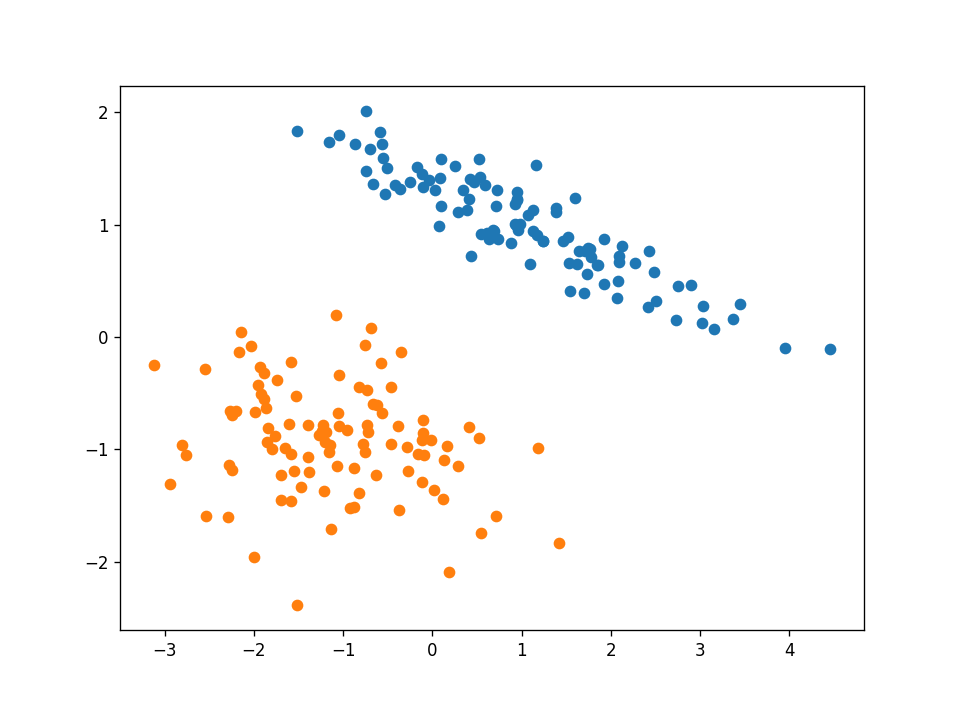
This is a simple dataset, and our perceptron algorithm will converge to a solution subsequently only 2 iterations through the grooming fix. And so, the animation frames volition change for each information point. The green point is the one that is currently tested in the algorithm.

On this dataset, the algorithm had correctly classified both the training and testing examples.

Example 2 — Noisy dataset

What if the dataset is non linearly separable? What if the positive and negative examples are mixed upwards similar in the paradigm beneath?

Well, the perceptron algorithm will non be able to correctly classify all examples, but information technology will effort to discover a line that best separates them. In this example, our perceptron got a 88% test accuracy. The animation frames beneath are updated subsequently each iteration through all the grooming examples.

Instance 3 — Non-linear dataset

What well-nigh the below dataset?

It is separable, only clearly not linear. So you may remember that a perceptron would not exist skillful for this task. Simply the matter about a perceptron is that information technology's decision purlieus is linear in terms of the weights, not necessarily in terms of inputs. Nosotros can augment our input vectors ten so that they contain non-linear functions of the original inputs. For example, in add-on to the original inputs x1 and x2 we tin add the terms x1 squared, x1 times x2, and x2 squared.

The polynomial_features(X, p) function below is able to transform the input matrix X into a matrix that contains as features all the terms of a polynomial of caste p. It makes use of the polynom() function which computes a list of indices that represent the columns to be multiplied for obtaining the p-social club terms.

                      def            polynom(indices_list, indices, a, b, p):
            indices            =            [*indices]
            if            p            ==            0:
            indices_list.suspend(indices)
            return            
            for            i            in            range(a, b):
            indices.suspend(i)
            polynom(indices_list, indices, i, b, p-1)
            indices            =            indices[0:-ane]              def              polynomial_features(10, p):
              n, d              =              10.shape
              features              =              []
              for              i              in              range(i, p+1):
              l              =              []
              polynom(l, [], 0, d, i)
              for              indices              in              l:
              x              =              np.ones((north,))
              for              idx              in              indices:
              x              =              x              *              10[:, idx]
              features.append(x)
              return              np.stack(features, axis=ane)

For our example, we volition add degree 2 terms as new features in the X matrix.

          10            =            polynomial_features(X, 2)

Now, let's run into what happens during training with this transformed dataset:

Note that for plotting, nosotros used only the original inputs in society to go along information technology 2D. The decision boundary is even so linear in the augmented feature space which is 5D now. Simply when nosotros plot that decision boundary projected onto the original feature space it has a not-linear shape.

With this method, our perceptron algorithm was able to correctly classify both preparation and testing examples without any modification of the algorithm itself. All we inverse was the dataset.

With this feature augmentation method, we are able to model very circuitous patterns in our data by using algorithms that were otherwise just linear.

Only, this method is non very efficient. Imagine what would happen if we had m input features and we want to augment information technology with upward to 10-degree polynomial terms. Fortunately, this problem can be avoided using something called kernels. Simply that'southward a topic for some other article, I don't want to make this one too long.

I promise you lot establish this information useful and thanks for reading!

This commodity is too posted on my own website hither. Feel complimentary to have a wait!